Random walk on n dimensional chessboard

**Disclaimer** : this post also serves as an experiment on using MathJax for integration of math formulas in this blog.

Tomorrow I’ll take on an oral midterm on the Information Theory course I’m re-taking this year (since I, well… failed it last year).

This time, though, I’m pretty sure I have a better handle of the concepts.

To be sure that I was able to get my way through the subjects regarding the part of the course on data compression, I started abstracting the reasoning on the (already mastered) class exercises to more general cases.

One of these exercises involves the study of a simple Discrete Time Markov Chain, which describes the movement of the King on a 3x3 chessboard. The analysis is rather simple.
First of all, however, I have to credit most of the whole thing (except the actual calculations, and the generalization) to my IT professor.

The starting exercise

The King is able to move in any direction, but only one cell at a time. You may not move out of the chessboard, obviously, and you can’t stay still for a turn. We exploit the use of graphs to help us describe the problem, characterizing the vertices as the possible positions and the edges as the possible movements.

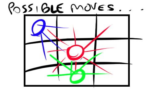
Possible moves of the king depending on the position.

Our king may move in 8 free directions if he’s at the center of the board (red), but only in 3 directions if he’s in a corner (blue), or 5 directions if he’s on the edge of the board (green).

Given that we’re analyzing a stationary and ergodic Markov Chain we have the whole thing very easy on us.

Using Flux balance analyisis we would be able to find the steady-state distribution, but it actually turns out that, since we are describing the problem through a non-oriented graph, each entry of the steady state distribution can be found as:

$$\mu_{i} = \dfrac{1}{2E}\sum_{j=1}^{M}{wji}$$

where:

• i,j stand as indexes for the position on the chessboard;
• $wji$ is the weight of the link between position i to j. It’s $wji =1$ for each edge since the King uses a uniform distribution when choosing where to move.
• $2E = \sum_{i=1}^{M}\sum_{j=1}^{M}{wji}$ is the sum of all the weights of the edges, which since are of unitary weight, turns out to be two times the sum of the edges (two times because each edge is counted both forward and backward), hence $2E$. In this case, its value is $2E = 4\cdot3 + 4\cdot5 + 8 = 40$
• $\mu_{i}$ is the probability of being in $i$-th state at steady-state distribution.

This is a very precious specialization which helps us avoid flux balance analyisis and its system of enormous quantity of linear equations to solve.

As one may easily notice, the steady state vector is:

$$\mu = \left(\dfrac{3}{2E}, \dfrac{5}{2E}, \dfrac{3}{2E}, \dfrac{5}{2E}, \dfrac{8}{2E}, \dfrac{5}{2E}, \dfrac{3}{2E}, \dfrac{5}{2E}, \dfrac{3}{2E}\right)$$

Entropy of Steady state distribution

When calculating entropy, not only the order does not matter (it’s an average), but we may also use a well-known trick, which is the Grouping rule for Entropy:

$$\begin{align} H(... , p_{i-1}, (p_{i}, ..., p_{j}), p_{j+1}, ...) = & H\left(... , p_{i-1}, p_{j+1}, ..., \sum_{k=i}^{j}{p_{k}}\right) + \\\\ & + \sum_{k=i}^{j}{p_{k}} \cdot H\left(p_{i} \cdot \sum_{k=i}^{j}{p_{k}}, ..., p_{j}\cdot\sum_{k=i}^{j}{p_{k}}\right) \end{align}$$

Sorry about the messy notation.
The trick means that the entropy of the vector can be calculated “extracting” a group $(p_{i}, ... , p_{j})$ and calculating its entropy “individually” following this rules, to simplify calculations (or, well, to prove stuff).

Now, applying the Grouping rule, we find:

$$\begin{align} H(\mu) & = H\left(\dfrac{3\cdot4}{2E},\dfrac{5\cdot4}{2E},\dfrac{8}{2E}\right) + \dfrac{3\cdot4}{2E} \log_{2}{4} + \dfrac{5\cdot4}{2E} \log_{2}{4} + \dfrac{8}{2E} log_{2}{1} \\\\ & = H\left(\dfrac{12}{40},\dfrac{20}{40},\dfrac{8}{40}\right) + \dfrac{12}{40} \cdot 2 + \dfrac{20}{40} \cdot 2 + 0 \\\\ & = H\left(\dfrac{3}{10},\dfrac{1}{2},\dfrac{1}{5}\right) + \dfrac{3}{5} + 1 \\\\ & = 3.085 (bit) \end{align}$$

Entropy Rate

We now seek the Entropy Rate of the process.
Given that we are dealing with a stationary and ergodic DTMC, it is very easy to find, by total probability.

$$H(\chi) = H(X2|X1) = \sum_{i=1}^{M}{H(\underline{ p }_{i})\cdot \mu_{i}}$$

where $H(\underline{ p }_{i})$ is the entropy of the $i$-th column of the transition matrix. We did not define such matrix, but it’s easy to see that the transition columns are all PMFs with uniform distribution:

• Four PMFs corresponding to the corners, with uniform distribution over 3 possible directions.
• Four PMFs corresponding to the edges, with uniform distribution over 5 possible directions.
• One PMF corresponding to the central position, with uniform distribution over 8 possible directions.

We already had the $\mu$, now we also have defined all the columns so we have everything that we need.

$$\begin{align} H(\chi) &= \dfrac{4\cdot3}{40} log_{2}{3} + \dfrac{4\cdot5}{40} log_{2}{5} + \dfrac{8}{40} log_{2}{8} \\\\ & = 2.24 (bit) \end{align}$$

As one would normally expect, the Entropy Rate is lower than the Entropy of the Steady state distribution.
However, this limited example, I thought, may not give an accurate idea of how this may impact our lives. I wanted some down-to-earth meaning.
Okay, it’s probably not actually going to change our life, but it can help a student give a meaning to what he’s doing. So here’s a different scenario.

Generalization to the case of a map of size NxN

We’re making an online game. We’re making it with limited resources.
Hella limited.
No, we don’t care about the fact that everyone has large bandwidth nowadays. We’re making a text-based online game in the late 80s/early 90s. We want our game to be played in a big (NxN) map, and we want our players to move through it. Each time we send and receive packets from server to players, we are occuping some bandwidth accordingly to the amount of info transmitted. We want to transmit as little information as possible, keeping however the game playable in the same way.

How do we transmit the positions of players?

Now, you already may know the answer, as we caught a glimpse of it in the previous exercise.
Let’s suppose we have $N=3$ as in the previous case. At Steady state, the amount of entropy regarding the position of a “player” on that little chessboard amounts to more than 3 bits. Ie, I need at least 4 bits (the closest bigger integer) to fully represent the position of the player in the map, and if I choose transmit these “absolute” values, I’m transmitting 4 bits per player in each packet. Yikes.

If I just choose to transmit the “direction” of the movement instead, given that I already knew the position of the player, I have 2.24 bits of uncertainty, which means I can use “just” 3 bits (the closest bigger integer). Not a big improvement, to be honest.

How does this change as the value of N reaches higher and higher values, approaching infinity?
Let’s see.

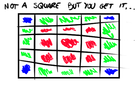
Sorry for this ugly ass picture.

• In red we have the inner cells, from which a player can move in 8 directions. They form an inner square, and they are $(N-2)^{2}$.
• In green we have the edge cells, which are $4 \cdot (N-2)$ since we are excluding the corners.
• In blue, we have the corners. Just 4 corners. Nothing new here.

We calculate $2E = 8\cdot(N-2)^2 + 5\cdot 4(N-2) + 3 \cdot 4$.

Repeating calculations for the Steady state distribution, we get a vector which is made of:

• $(N-2)^2$ entries of the kind $\dfrac{8}{2E}$;
• $4\cdot(N-2)$ entries of the kind $\dfrac{5}{2E}$;
• $4$ entries of the kind $\dfrac{3}{2E}$;

Applying Grouping rule when calculating Entropy of the Steady state distribution:

$$\begin{align} H(\mu) = & H\left(\dfrac{12}{2E},\dfrac{4\cdot5\cdot(N-2)}{2E}, \dfrac{8\cdot(N-2)^2}{2E}\right) + \dfrac{12}{2E}\cdot log_{2}{4} + \\\\ & + \dfrac{3\cdot4}{2E}\cdot log_{2}{(4\cdot(N-2))} + \dfrac{8\cdot(N-2)^{2}}{2E}\cdot log_{2}{(N-2)^{2}} \end{align}$$

Can’t simplify more than that.
We can however look for the Entropy Rate, now.

$$\begin{align} H(\chi) &= \sum_{i=1}^{N^2}{H(\underline{ p }_{i})\cdot \mu_{i}} \\\\ & = \dfrac{3\cdot4}{2E} log_2{3} + \dfrac{5\cdot4\cdot(N-2)}{2E}log_{2}{5} + \dfrac{8\cdot(N-2)^2}{2E}log_2{8} \end{align}$$

At this point we can make a comparison of these two quantities as $N\to\infty$. Since $2E \sim \mathcal{O}((N-2)^2)$, we have:

$$\begin{align} H(\mu) &\sim \mathcal{O}\left(\dfrac{(N-2)^2}{(N-2)^2} \cdot 2log_{2}{(N-2)}\right) \\\\ & \sim \mathcal{O}(2log_{2}{(N-2)}) \\\\ & \sim \mathcal{O}(2log_{2}{(N)}) \end{align}$$

However, something different applies to $H(\chi)$:

$$\begin{align} H(\mu) &\sim \mathcal{O}\left(\dfrac{(N-2)^2}{(N-2)^2}\right) \\\\ & \sim \mathcal{O}(1) \end{align}$$

This was a predictable result, but I think it was well worth the analysis.

If you’re trying to transmit absolute positions, be ready to pay the bit price, as the size of the map increases.
A differential encoding, instead, ensures that even for a large map (very intuitively) you don’t need as many bits, given that you transmit the absolute position of the players just one time, at the start of the game.

Hooray for this small source compression result. The main thing that I liked about this result is that it’s a very easy, yet efficient way to prove mathematically what would be otherwise just an intuition for optimization.

Now, off to revising, otherwise I’m doomed.

Meru.